Using spreadsheets in Impress
A
spreadsheet embedded in Impress includes most of the functionality
of a spreadsheet in Calc and is therefore capable of performing
extremely complex calculations and data analysis. However, in most
cases people limit the use of spreadsheets in Impress to creating
complex tables or presenting data in a tabular format. If you need
to analyse your data or apply formulas, these operations are best
performed in a Calc spreadsheet and the results displayed in an
embedded Impress spreadsheet.
Inserting
a spreadsheet
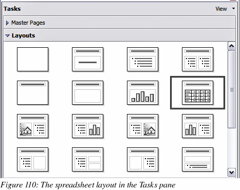
To
add a spreadsheet to a slide, select the corresponding layout in the
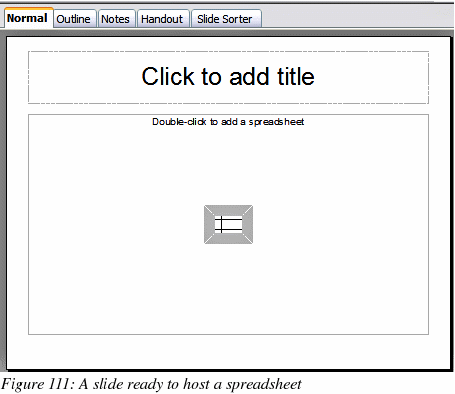
list of predefined layouts in the Tasks pane, as shown in Figure 110.
This inserts a placeholder for a spreadsheet in the center of a
slide, as shown in Figure 111. To insert data and modify the
formatting of the spreadsheet, it is necessary to activate
it and enter the edit mode. To do so, double-click inside the frame
with the green handles.
Alternatively,
select Insert >
Spreadsheet from the main menu bar. This opens a small
spreadsheet in the middle of the slide. When a spreadsheet is
inserted using this method, it is already in edit mode.
It
is also possible to insert a spreadsheet as an OLE object as
described in “Inserting other objects” on page 164.
When
editing a spreadsheet, some of the contents of the main menu bar
change, as does the Formatting toolbar (see Figure 112), to show
entries and tools that support working with the spreadsheet.
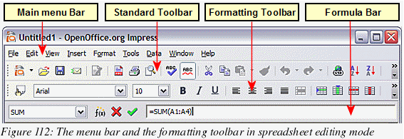
One
of the most important changes is the presence of the Formula
toolbar, just below the Formatting toolbar. The Formula toolbar
contains (from left to right):
The active cell
reference or the name of the selected range
The
Formula Wizard button
The
Sum and Formula buttons or
the Cancel and Accept buttons (depending on the contents of the
cell)
A
long edit box to enter or review the contents of a cell
If
you are familiar with Calc, you will immediately recognize the tools
and the menu items since they are much the same.
Resizing
and moving a spreadsheet
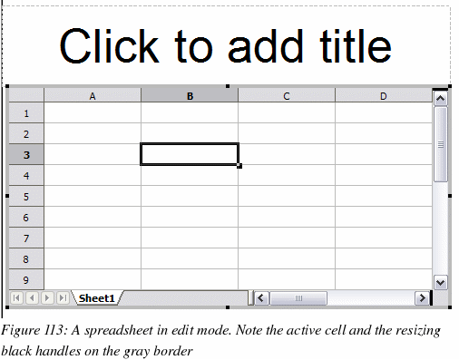
To
resize the area occupied by the spreadsheet or change its position,
enter the edit mode and use the black handles found in the gray
border surrounding the spreadsheet (see Figure 113).
Move
the mouse over the handles to resize the spreadsheet area. The
corner handles resize the two sides forming the corner
simultaneously, while the handles in the middle of the sides modify
one dimension at a time. When moved over each handle, the cursor
changes shape to give a visual representation of the effects applied
to the area.
When
resizing or moving a spreadsheet, ignore the first row and the first
column (easily recognizable because of their light gray background)
and the horizontal and vertical scroll bars). They are only used for
editing purposes and will not be included in the visible area of the
spreadsheet on the slide.
The
position of the spreadsheet within the slide can be changed both
when in edit mode and when not in edit mode. In both cases:
Move
the mouse over the border until the cursor changes shape (typically
a four-headed arrow).
Click
the left mouse button and drag the spreadsheet to the desired
position.
Release
the mouse button.
When
not in edit mode (green handles), the spreadsheet object is treated
like any other object, therefore resizing it results in changing the
scale rather than the spreadsheet area. This is not recommended as
it may produce distortion of the fonts and picture shapes.
Moving
around the spreadsheet and entering data
How
a spreadsheet is organized
A
spreadsheet consists normally of multiple tables which in turn
contain cells. However, in Impress only one of these tables can be
shown at any given time on a slide.
The
default for a spreadsheet embedded in Impress is one single table
called “Sheet 1”. The name of the table is shown at the bottom
of the spreadsheet area (see Figure 113).
If
required, it is possible to add other sheets. To do that:
Right-click
on the bottom area.
Select
Insert > Sheet
from the pop-up menu.
Just
like in Calc, it is possible to rename a sheet or move it to a
different position using the same pop-up menu or the Insert
menu in the main menu bar.
|
Note
|
Even
if you have many sheets in your embedded spreadsheet, only the
sheet which is active when leaving the spreadsheet edit mode will
be shown on the slide.
|
Each
of the sheets is further organized in cells.
Cells are the elementary unit of the spreadsheet. They are
identified by a row number (shown on the left hand side on gray
background) and a column letter (shown in the upper part again on
gray background). For example, the top left cell is identified as
A1, while the third cell on the second row is C2. All data, whether
text or numbers, is input in a cell.
Moving
the cursor to a cell
To
move around the spreadsheet and select the cell which has the focus,
you can:
Use the arrow
keys.
Left-click
with the mouse on the desired cell.
Use
the combinations Enter
and Shift+Enter
to move one cell down or one cell up respectively; Tab
key and Shift+Tab
key to move one cell to the right or to the left respectively.
Other
keyboard shortcuts are available to move quickly to certain cells of
the spreadsheet. Refer to Chapter 7 (Getting Started with Calc) in
the Getting
Started guide for further information.
Entering
data in the selected cell
Keyboard
input is received by the active
cell, identified by a thick black border (see Figure 113 where cell
B3 is active). The cell reference (or “coordinates”) is also
shown on the left hand end of the formula bar.
To
insert data, first select the cell to make it active, then type in
it. Note that the input is also added to the main part of the
formula bar where it may be easier to read.
Impress
will try to automatically recognize the type of contents (text,
number, date, time and so on) of a cell and apply default formatting
to it. Note how the formula bar icons change according to the type
of input, displaying accept and reject buttons ( )
whenever the input is not a formula. Use the green Accept button to
accept the input made in a cell or simply select a different cell.
In case Impress wrongly recognized the type of input, it is possible
to change it using the toolbar shown in Figure 112, or from the
Format > Cells
in the main menu bar.
)
whenever the input is not a formula. Use the green Accept button to
accept the input made in a cell or simply select a different cell.
In case Impress wrongly recognized the type of input, it is possible
to change it using the toolbar shown in Figure 112, or from the
Format > Cells
in the main menu bar.
|
Tip
|
Sometimes
it is useful to treat numbers as text (for example, telephone
numbers) and to prevent Impress from removing the leading zeros
or right align them in a cell. To force Impress to treat the
input as text, type a single apostrophe
' (U + 00B4) before entering the number.
|
Formatting
spreadsheet cells
Normally,
for the purpose of a presentation it may be necessary to increase
considerably the size of the font as well as matching it to the
style used in the presentation.
The
fastest and most flexible way to format the embedded spreadsheet is
to make use of styles. When working on an embedded spreadsheet it is
possible to access the cell styles created in Calc and use them. It
is however recommended to create specific cell styles for
presentation spreadsheets, as the Calc cell styles are likely to be
unsuitable when working within Impress.
To
apply a style (or indeed manual formatting of the cell attributes)
to a cell or group of cells simultaneously, first select the range
to which the changes will apply. A range consists of one or more
cells, normally forming a rectagular area. A selected range
consisting of more than one cell can be easily recognized because
all its cells except the active one have a black background. To
select a multiple cells range:
Click
on the first cell belonging to the range (either the left top cell
or the right bottom cell of the rectangular area).
Keep
the left mouse button pressed and move the mouse to the opposite
corner of the rectangular area which will form the selected range.
Release
the mouse button.
To
add further cells to the selection press the Control
key and repeat the steps 1 to 3 above.
|
Tip
|
You
can also click on the first cell in the range, hold down the
Shift
key, and click in the cell in the opposite corner. Refer to
Chapter 7 (Getting Started with Calc) in the Getting
Started
book for further information on selecting ranges of cells.
|
Some shortcuts are
very useful to speed up the selection:
To
select the whole visible sheet, click at the intersection between
the rows indexes and the column indexes, or press Control+A.
To
select a column, click on the column index at the top of the
spreadsheet.
To
select a row, click on the row index on the left hand side of the
spreadsheet.
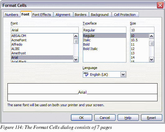
Once
the range is selected, you can modify the formatting such as font
size, alignment (including vertical alignment), font color, number
formats, borders, background and so on. To access these settings,
select Format > Cells
from the main menu bar. This command opens the dialog shown in Figure 114.
If
the text does not fit the width of the cell, increase these values
by hovering the mouse over the line separating two columns and, when
the mouse cursor changes shape, clicking the left button and
dragging the separating line to the new position. A similar
procedure can be used to modify the height of a cell (or group of
cells).
To
insert rows and columns in a spreadsheet, use the Format
menu or right-click on the row and column headers and select the
appropriate option from the pop up menu. To merge multiple
cells, select the cells to be merged and select Format
> Merge cells from the main menu bar. To de-merge a
group of cells, select the group and again Format
> Merge Cells (which will now have a checkmark next to
it).
When
you are satisfied with the formatting and the appearance of the
table, exit the edit mode by clicking outside the spreadsheet area.
Note that Impress will display exactly the section of the
spreadsheet which was on the screen before leaving the edit mode.
This allows you to hide additional data from the view, but it may
cause the apparent loss of rows and columns. Therefore, take care
that the desired part of the spreadsheet is showing on the screen
before leaving the edit mode.