Operators in formulas
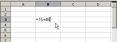
Each cell on the worksheet can be used as a data holder or a place for data calculations. Inserting data is accomplished simply by typing the data in the cell and moving to the next cell or pressing Enter. With formulas the equal sign denotes that instead of the cell being a data holder, the cell will be used for a calculation. A mathematical calculation like 15 + 46 can be accomplished as shown below.
 | To enter the = symbol for a purpose other than creating a formula as described in this chapter, type an apostrophe or single quotation mark before the data; for example, '= means different things to different people. Calc treats everything after the single quotation symbol as text.
|
| Simple Calculation in 1 Cell
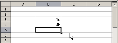
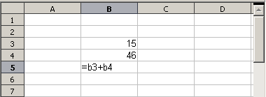
| Calculation by Reference
|
|
|
|
|
|
|
|
A simple calculation.
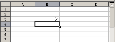
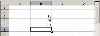
While the calculation on the left was accomplished in only one cell, the real power is shown on the right where the data is placed in cells and the calculation is performed using references back to the cells. In this case, cells B3 and B4 were the data holders with B5 the cell where the calculation was performed. Notice that the formula was shown as =B3 + B4. The plus sign denotes addition as the operation being performed upon the data within cells B3 and B4. All formulas build upon this concept. Other ways of entering formulas are shown in Table 1.
These back references to find data to perform a calculation can be found anywhere in the worksheet being worked on or upon any other worksheet in the workbook that is opened. If the data needed was on different worksheets they would be referenced by referring to the worksheet, for example =SUM(Sheet2.B12+Sheet3.A11).
Table 1: Common ways to enter formulas.
| Formula
| Description
|
| =A1+10
| Displays the contents of cell A1 plus 10.
|
| =A1*16%
| Displays 16% of the contents of A1.
|
| =A1 * A2
| Displays the result of the multiplication of A1 and A2.
|
| =ROUND(A1;1)
| Displays the contents of cell A1 rounded to one decimal place.
|
| =EFFECTIVE(5%;12)
| Calculates the effective interest for 5% annual nominal interest with 12 payments a year.
|
| =B8-SUM(B10:B14)
| Calculates B8 minus the sum of the cells B10 to B14.
|
| =SUM(B8;SUM(B10:B14))
| Calculates the sum of cells B10 to B14 and adds the value to B8.
|
| =SUM(B1:B65536)
| Sums all numbers in column B.
|
| =AVERAGE(BloodSugar)
| Displays the average of a named range defined under the name BloodSugar.
|
| =IF(C31>140; "HIGH"; "OK")
| Displays the results of a conditional analysis of data from two sources. If C31 = 144, then HIGH is displayed, otherwise OK is displayed.
|
|
| Users of Lotus 1-2-3®, Quattro Pro® and other spreadsheet software may be familiar with formulas that begin with +, -, =, (, @, ., $, or </nowiki>#. A mathematical formula would look like +D2+C2 or +2*3. Functions begin with the <nowiki>@ symbol such as @SUM(D2..D7), @COS(@DEGTORAD(30)) and @IRR(GUESS;CASHFLOWS). Ranges are identified such as A1..D3.
|
Functions can be identified in Table 1 with a word, for example ROUND, followed by parentheses enclosing references or numbers.
It is also possible to establish ranges for inclusion by naming them using Insert > Names, for example BloodSugar representing a range such as B3:B10. Logical functions can also be performed as represented by the IF statement which results in a conditional response based upon the data in the identified cell.