Operator types
You can use the following operators in OpenOffice.org Calc: arithmetic, comparative, descriptive, text, and reference.
Arithmetic operators
The addition, subtraction, multiplication and division operators return numerical results. The Negation and Percent operators identify a characteristic of the number found in the cell, for example -37. The example for Exponentiation illustrates how to enter a number that is being multiplied by itself a certain number of times, for example 23 = 2*2*2.
Table 2: Arithmetical operators
| Operator
| Name
| Example
|
| + (Plus)
| Addition
| =1+1
|
| - (Minus)
| Subtraction
| =2-1
|
| - (Minus)
| Negation
| -5
|
| * (asterisk)
| Multiplication
| =2*2
|
| / (Slash)
| Division
| =10/5
|
| % (Percent)
| Percent
| 15%
|
| ^ (Caret)
| Exponentiation
| 2^3
|
Comparative operators
Comparative operators are found in formulas that use the IF function and return either a true or false answer; for example, =IF(B6>G12; 127; 0) which, loosely translated, means if the contents of cell B6 are greater than the contents of cell G12, then return the number 127, otherwise return the number 0.
A direct answer of TRUE or FALSE can be obtained by entering a formula such as =B6>B12. If the numbers found in the referenced cells are accurately represented, the answer TRUE is returned, otherwise FALSE is returned.
Table 3: Comparative operators
| Operator
| Name
| Example
|
| = (equal sign)
| Equal
| A1=B1
|
| > (Greater than)
| Greater than
| A1>B1
|
| < (Less than)
| Less than
| A1<B1
|
| >= (Greater than or equal to)
| Greater than or equal to
| A1>=B1
|
| <= (Less than or equal to)
| Less than or equal to
| A1<=B1
|
| <> (Inequality)
| Inequality
| A1<>B1
|
Descriptive operators
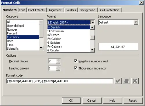
Currency symbols are perhaps the most commonly used descriptive operators found in Calc. Calc handles as currency an amount like $0.97 or £0.97 entered into a cell formatted as general or currency. However, it does not handle other currency types entered in this fashion. For other currencies, it is best to format the cells as the specific currency type, such as Yen (¥). To do this, right-click on the affected cells and select Formatting Cells. On the tab Numbers tab, select Currency. In the Format list, select the appropriate currency type.
When entering amounts, it is not necessary to enter a currency symbol. Some currency symbols such as the Yen may not display.
Currency symbols.
 | Users experienced in the use of an adding machine may experience difficulty with data entry, with resulting loss of data or incorrect results displaying. Adding machine users typically enter numbers from left to right without entering a decimal point. For example, the entry of 97 will display as 0.97. In cells formatted as currency, the entry of 97 will display currency for the locale selected such as $97 or £97, not $0.97 or £0.97.
|
Text operators
It is common for users to place text in spreadsheets. To provide for variability in what and how this type of data is displayed, text can be joined together in pieces coming from different places on the spreadsheet. Below is an example.
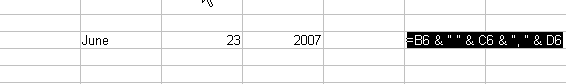
Text Concatenation.
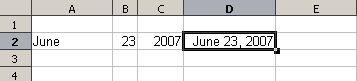
In this example, specific pieces of the text were found in three different cells. To join these segments together, the formula also adds required spaces and punctuation housed within quotation marks resulting in a formula of =B6 & " " & C6 & ", " D6. The result is the concatenation into a correctly formatted date for this locale.
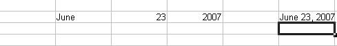
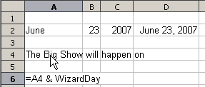
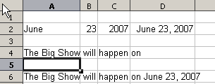
Taking this example further, the result cell is defined as a name, then text concatenation is performed using this defined name.
Defining a name for a range of cells.
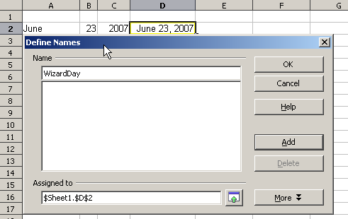
Naming a cell or range of cells for inclusion in a formula.
Defining Names on a worksheet.
Reference operators
Reference operators merge the values held in each individual cell within the range. Reference operators can be an individual cell identified by the column identifier located along the upper edge of the spreadsheet and a numeric identifier found along the side of the spreadsheet. On spreadsheets read from left to right, the upper left cell is A1. The figure below shows these identifiers for Cell A1.
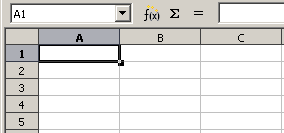
The Cell Reference Operator.
A range is also a reference operator referenced in formulas, functions and logical operators. The range for left to right operations refers to the upper left cell running to the right and downward to the right bottommost cell as shown below.
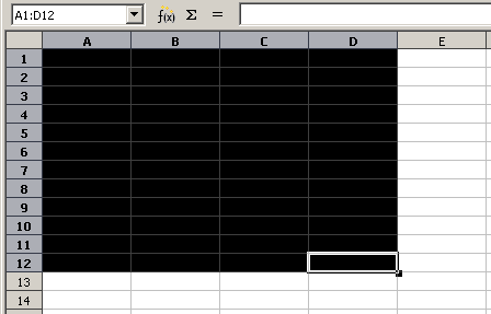
Reference Operator for a range.
In the upper left corner of the figure above, the range A1:D12 is shown, corresponding to the cells included in the drag operation with the mouse to highlight the range. This same range could also be created by entering in the Name Box directly as shown below. After pressing Enter, the same range is selected.
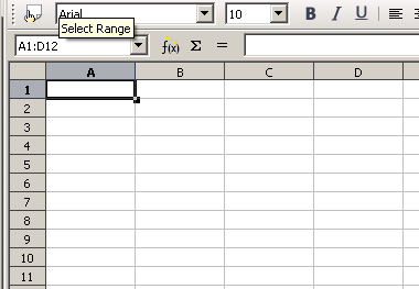
Direct entry of Reference Operator into Name Box.
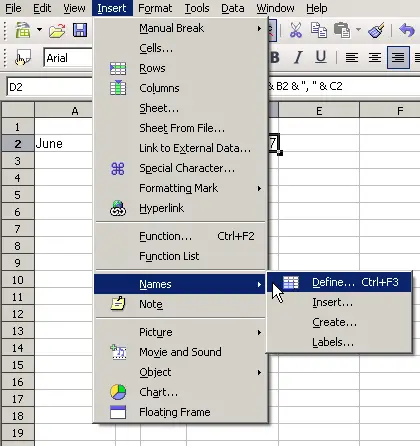
A reference operator can also be created by defining a named area by selecting the menu item Insert > Names > Define, pressing Ctrl+F3, or clicking the icon, if it shows on your toolbar.
Another reference operator involves the use of the '!' sign. If data appears in range A1:B6 as well as range B5:C12, using a formula such as SUM(A1:B6!B5:C12) will yield the sum of cells B5 and B6.